TL; DR
This document demonstrates how to modify the algorithm used for inference in our models. In general, the default algorithm (the NUTS from Stan) represents the gold standard, but it is slow. For initial screening (or even cross-validation), one can rely on the other algorithms showcased in this vignette. They tend to be faster, and produce reliable point estimates but have a weaker performance in quantifying the uncertainty around their estimates.
Setup
The setup and data-processing for this vignette is the same as in the “Advanced features” vignette. For further details, see vignette("advanced-features", "drmr"). Unlike the examples in that vignette, we will not split the data into train and test, but rather just look at parameters’ estimates obtained through different algorithms.
Linking to GEOS 3.12.1, GDAL 3.8.4, PROJ 9.4.0; sf_use_s2() is TRUE
This is bayesplot version 1.15.0
- Online documentation and vignettes at mc-stan.org/bayesplot
- bayesplot theme set to bayesplot::theme_default()
* Does _not_ affect other ggplot2 plots
* See ?bayesplot_theme_set for details on theme setting
Attaching package: 'dplyr'
The following object is masked from 'package:drmr':

    between
The following objects are masked from 'package:stats':

    filter, lag
The following objects are masked from 'package:base':

    intersect, setdiff, setequal, union
## loads the data
data(sum_fl)

## computing density
sum_fl <- sum_fl |>
  mutate(dens = 100 * y / area_km2,
         .before = y)

avgs <- c("stemp" = mean(sum_fl$stemp),
          "btemp" = mean(sum_fl$btemp),
          "depth" = mean(sum_fl$depth),
          "n_hauls" = mean(sum_fl$n_hauls),
          "lat" = mean(sum_fl$lat),
          "lon" = mean(sum_fl$lon))

min_year <- sum_fl$year |>
  min()

## centering covariates
sum_fl <- sum_fl |>
  mutate(c_stemp = stemp - avgs["stemp"],
         c_btemp = btemp - avgs["btemp"],
         c_hauls = n_hauls - avgs["n_hauls"],
         c_lat   = lat - avgs["lat"],
         c_lon   = lon - avgs["lon"],
         time  = year - min_year)

## mortality rates
fmat <-
  system.file("fmat.rds", package = "drmr") |>
  readRDS()

shp_sum_fl <- system.file("maps/sum_fl.shp", package = "drmr") |>
  st_read()
Reading layer `sum_fl' from data source
  `/home/runner/work/_temp/Library/drmr/maps/sum_fl.shp' using driver `ESRI Shapefile'
Simple feature collection with 10 features and 3 fields
Geometry type: MULTIPOLYGON
Dimension:     XY
Bounding box:  xmin: -75.77033 ymin: 35.18407 xmax: -65.67583 ymax: 44.4013
Geodetic CRS:  WGS 84
For an extensive list of the variables present in this dataset run: ?sum_fl.
Fitting a model using different algorithms
We will start with the default algorithm (NUTS). By default, it runs 4 chains sequentially, with a warmup period od 1000 samples and, subsequently, 1000 samples per chain. Here, we are running two chains in parallel, with a warmup of 500 and drawing 500 samples.
nuts_args <- list(parallel_chains = 2,
                  chains = 2,
                  iter_sampling = 500,
                  iter_warmup = 500,
                  show_messages = FALSE,
                  show_exceptions = FALSE)

drm_nuts <-
  fit_drm(.data = sum_fl,
          y_col = "dens", ## response variable: density
          time_col = "year", ## vector of time points
          site_col = "patch",
          family = "gamma",
          seed = 2026,
          formula_zero = ~ 1 + c_hauls,
          formula_rec = ~ 1 + c_stemp + I(c_stemp * c_stemp),
          formula_surv = ~ 1,
          f_mort = fmat[, -1],
          n_ages = NROW(fmat),
          adj_mat = adj_mat, ## A matrix for movement routine
          ages_movement = c(0, 0,
                            rep(1, 12),
                            0, 0), ## ages allowed to move
          .toggles = list(ar_re = "rec",
                          movement = 1,
                          est_surv = 1,
                          est_init = 0,
                          minit = 1),
          algo_args = nuts_args)
Warning: 1 of 1000 (0.0%) transitions ended with a divergence.
See https://mc-stan.org/misc/warnings for details.
Next, we obtain samples from the variational posterior using Stan’s Automatic Differentiation Variational Inference (ADVI) algorithm (for for details see this link).
advi_args <- list(show_messages = FALSE,
                  show_exceptions = FALSE,
                  iter = 10^5, ## maximum number of iterations (optimization)
                  draws = 4000) ## number of samples from the posterior

drm_advi <-
  fit_drm(.data = sum_fl,
          y_col = "dens", ## response variable: density
          time_col = "year", ## vector of time points
          site_col = "patch",
          family = "gamma",
          seed = 2026,
          formula_zero = ~ 1 + c_hauls,
          formula_rec = ~ 1 + c_stemp + I(c_stemp * c_stemp),
          formula_surv = ~ 1,
          f_mort = fmat[, -1],
          n_ages = NROW(fmat),
          adj_mat = adj_mat, ## A matrix for movement routine
          ages_movement = c(0, 0,
                            rep(1, 12),
                            0, 0), ## ages allowed to move
          .toggles = list(ar_re = "rec",
                          movement = 1,
                          est_surv = 1,
                          est_init = 0,
                          minit = 1),
          algo_args = advi_args,
          algorithm = "vb") ## vb stands for variational Bayes
Another algorithm option is the Pathfinder. Pathfinder also relies on variational inference. It is usually better than ADVI, especially when the posteriors (in the unconstrained space) are not unimodal and bell-shaped. We will demonstrate how the inference algorithm can be updated using the update method:
path_args <- list(show_messages = FALSE,
                  show_exceptions = FALSE,
                  max_lbfgs_iters = 10^4)

drm_path <-
  update(drm_advi,
         algo_args = path_args,
         algorithm = "pathfinder")
Optimization terminated with error: Line search failed to achieve a sufficient decrease, no more progress can be made Stan will still attempt pathfinder but may fail or produce incorrect results.
Only 3 of the 4 pathfinders succeeded.
Pareto k value (2) is greater than 0.7. Importance resampling was not able to improve the approximation, which may indicate that the approximation itself is poor.
It is also possible to obtain samples from a Laplace approximation of the posterior as follows:
lapl_args <- list(show_messages = FALSE,
                  show_exceptions = FALSE)

drm_lapl <-
  update(drm_path,
         algo_args = lapl_args,
         algorithm = "laplace")
Rejecting initial value:
  Log probability evaluates to log(0), i.e. negative infinity.
  Stan can't start sampling from this initial value.
Rejecting initial value:
  Log probability evaluates to log(0), i.e. negative infinity.
  Stan can't start sampling from this initial value.
Rejecting initial value:
  Log probability evaluates to log(0), i.e. negative infinity.
  Stan can't start sampling from this initial value.
Initial log joint probability = -41305.8
    Iter      log prob        ||dx||      ||grad||       alpha      alpha0  # evals  Notes
Exception: Exception: gamma_lpdf: Inverse scale parameter[1] is inf, but must be positive finite! (in '/tmp/Rtmp7kQpBr/pkg-lib1be17e389576/drmr/bin/stan/utils/lpdfs.stan', line 97, column 4, included from
'/tmp/Rtmp8LMTQe/model-2afb13976e39.stan', line 2, column 0) (in '/tmp/Rtmp8LMTQe/model-2afb13976e39.stan', line 312, column 2 to line 315, column 67)
Error evaluating model log probability: Non-finite gradient.
      99       63.1399     0.0384463       27.1111      0.2853      0.2853      137
    Iter      log prob        ||dx||      ||grad||       alpha      alpha0  # evals  Notes
     199       79.2643    0.00182743       12.9102      0.5695      0.5695      283
    Iter      log prob        ||dx||      ||grad||       alpha      alpha0  # evals  Notes
     299       81.6229     0.0254943       8.15253       1.395      0.1395      398
    Iter      log prob        ||dx||      ||grad||       alpha      alpha0  # evals  Notes
     399        82.725     0.0330018       3.68405           1           1      524
    Iter      log prob        ||dx||      ||grad||       alpha      alpha0  # evals  Notes
     499       83.1288    0.00405507       20.9462      0.9193      0.9193      644
    Iter      log prob        ||dx||      ||grad||       alpha      alpha0  # evals  Notes
     599       83.4274    0.00830204       7.15666           1           1      771
    Iter      log prob        ||dx||      ||grad||       alpha      alpha0  # evals  Notes
     699       83.4563    0.00924625       1.28662           1           1      898
    Iter      log prob        ||dx||      ||grad||       alpha      alpha0  # evals  Notes
     799       83.4863    0.00703205      0.672952           1           1     1017
    Iter      log prob        ||dx||      ||grad||       alpha      alpha0  # evals  Notes
     899       83.4936    0.00042654      0.290122      0.4865     0.04865     1146
    Iter      log prob        ||dx||      ||grad||       alpha      alpha0  # evals  Notes
     999       83.4947    0.00144258      0.217513       2.555      0.2555     1279
    Iter      log prob        ||dx||      ||grad||       alpha      alpha0  # evals  Notes
    1047        83.495   0.000179283     0.0613661      0.9495      0.9495     1340
Optimization terminated normally:
  Convergence detected: relative gradient magnitude is below tolerance
Finished in  0.8 seconds.
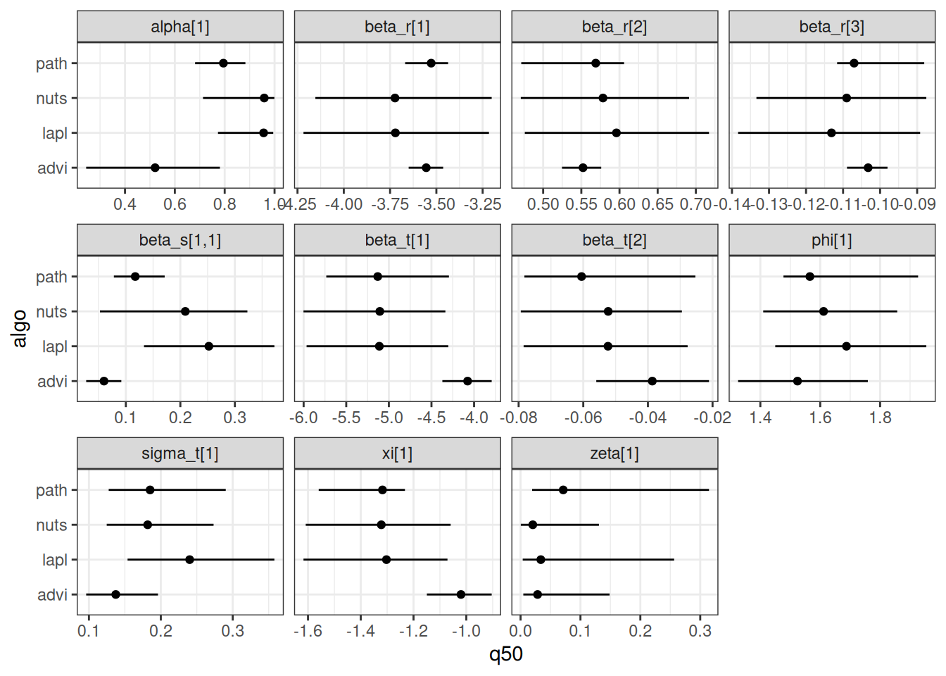
The code below computes the parameter estimates for each of the methods, and then makes a graph to compare them.
bind_rows(
    mutate(summary(drm_nuts)$estimates, algo = "nuts"),
    mutate(summary(drm_advi)$estimates, algo = "advi"),
    mutate(summary(drm_path)$estimates, algo = "path"),
    mutate(summary(drm_lapl)$estimates, algo = "lapl")
) |>
  ggplot(data = _,
         aes(x = q50,
             y = algo)) +
  geom_linerange(aes(xmin = q5, xmax = q95)) +
  geom_point() +
  facet_wrap(~ variable, scales = "free_x") +
  theme_bw()
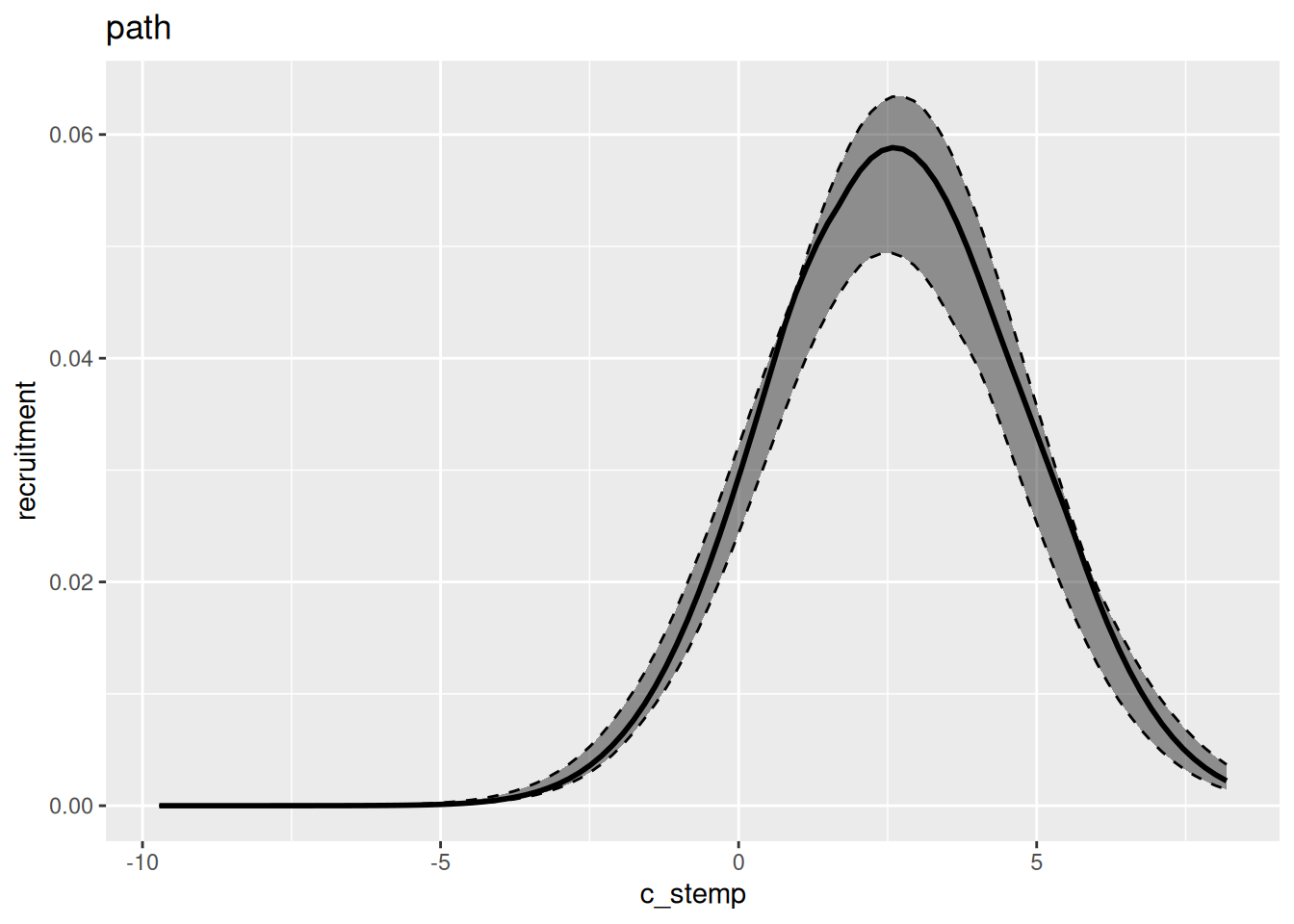
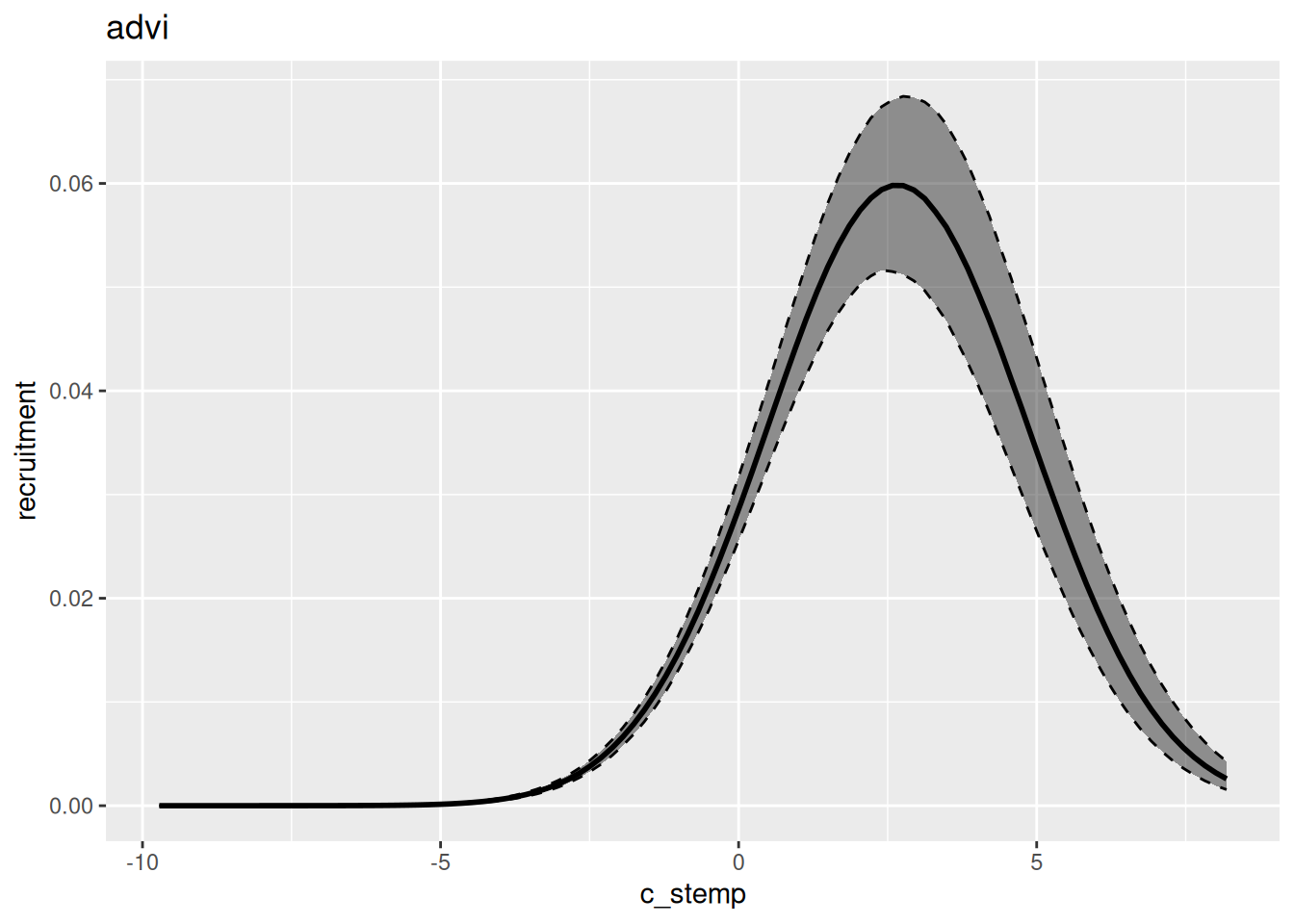
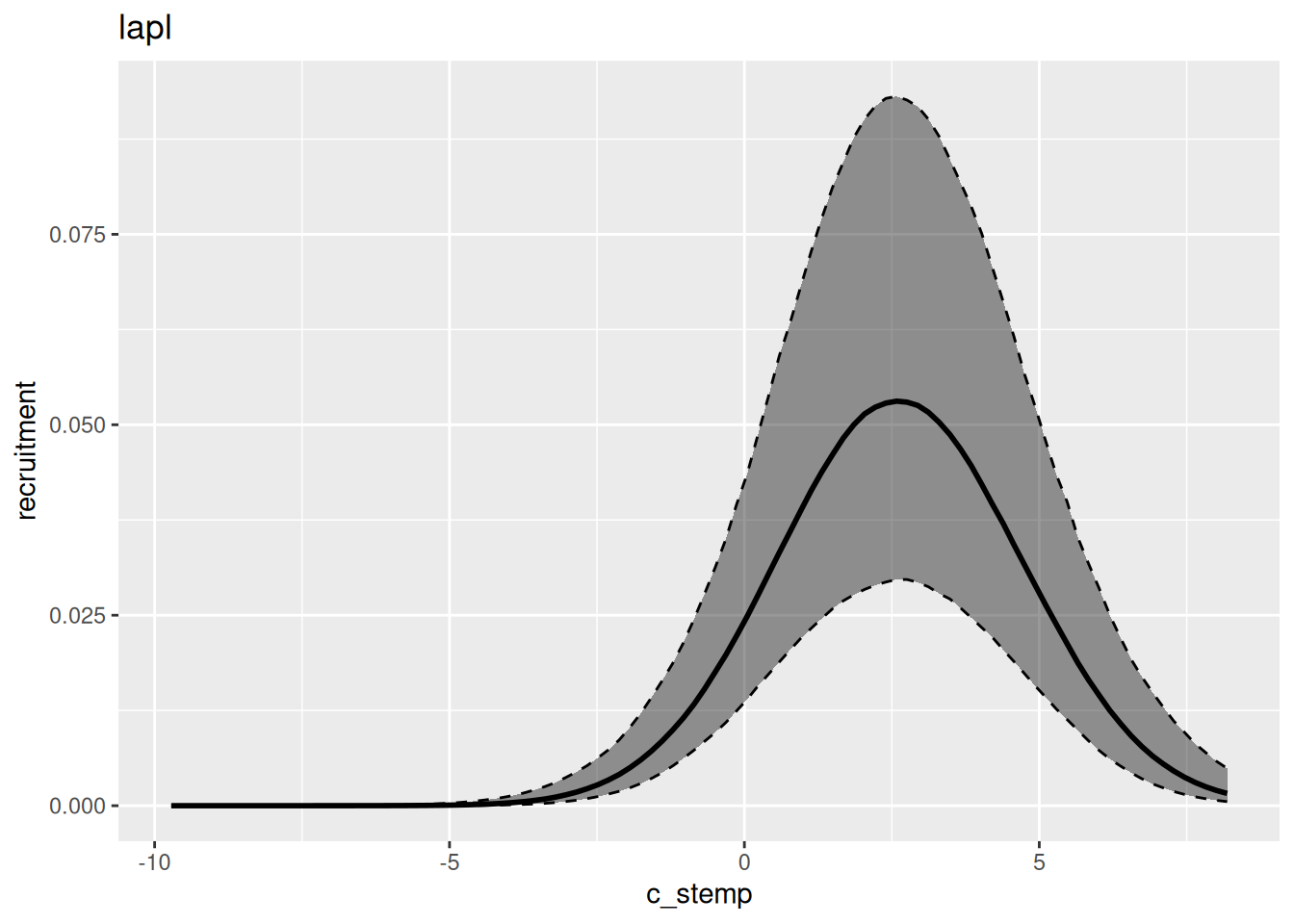
In general, variational inference methods are known for underestimating the uncertainty around the parameter estimates. We can also look at the estimated relationship between environment and recruitment for each of those methods: